Retrieval Augmented Generation (RAG)

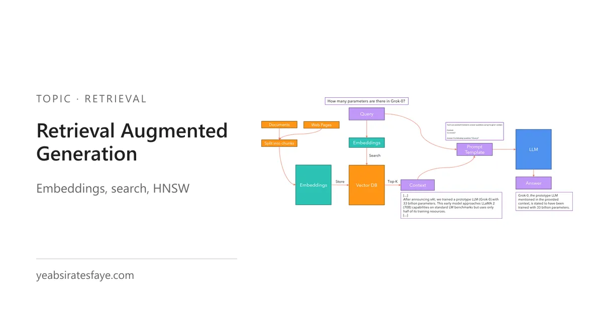
Welcome back, today we’ll raise the curtain of the one and only RAG and see the inner workings and algorithms behind the core ideas from first principle. RAG is a method of accessing and using external knowledge to help our LLM generate correct and accurate responses. It first starts with preparing our data and storing it. For example lets say our corpus is some proprietary documents and our website. We chunk both into smaller sizes.

We then convert our chunks into vector embeddings of same size. These vector embeddings represent the meaning of that chunk within the context and we store them in a vector database.

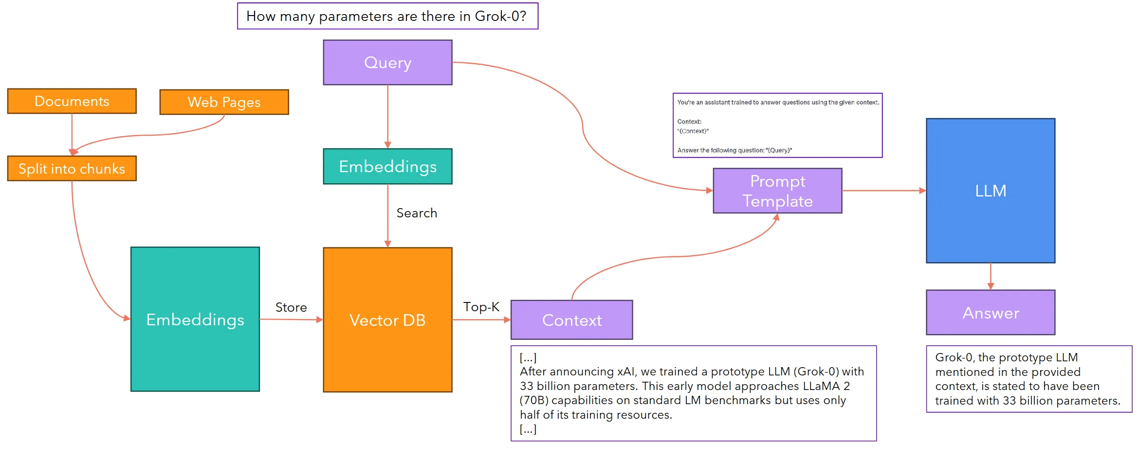
During inference, we use same embedding function to convert our query into an embedding, we then search that embedding from our database and filter out the top k similar embeddings and take their values and embed it in a prompt template which will be given to an LLM to generate an answer.

We can use models as BERT to generate our embedding so lets use it as an example and see how we train our embedding vectors using BERT. As we’ve discussed during our BERT note, it will take a tokens each represented by n dimension and after passing through the full encoder will give us tokens of n dimension but this time capturing both the meaning and the contextual information’s around. Then we take the avg over the whole tokens to get one vector representing a single vector.

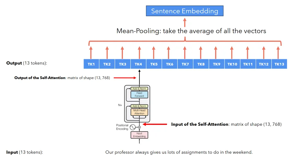
Now assuming we understood how we create the embedding vectors which will be used to represent both data stored in our database and our query, now lets see how we do searching and compare similarity.

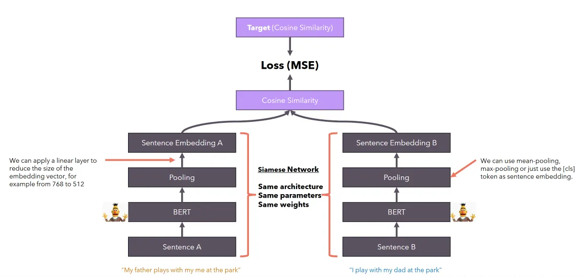
One of the ways to do comparison between embedding vectors is cosine similarity, which results higher similarity score for vectors close to each other(having closer meaning). But the thing is, BERT doesn’t know whether it has to represent similar concepts within close embedding dimensions so we need to teach it.

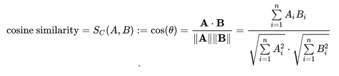
Lets look into Sentence-BERT, a work that introduces a clean way of teaching this similarity representation for BERT. Lets take two similar sentences as input, we first pass them through our BERT and then do the mean polling to capture the contextual understanding of each sentences and once we’ve the embedding for both sentences, we calculate the cosine similarity based on the embedding vector and compare it with our target cosine similarity and do Mean Square Error loss estimation and update our embedding vectors to represent this closeness.

Now lets talk about a vector database, how we add, search and retrieve from it.

While KNN(K nearest neighbor) search would have been the ideal, it takes huge compute time and resources to calculate distance between O(K*N) items so we need to find algorithms that approximate enough to trade off between speed for some accuracy.

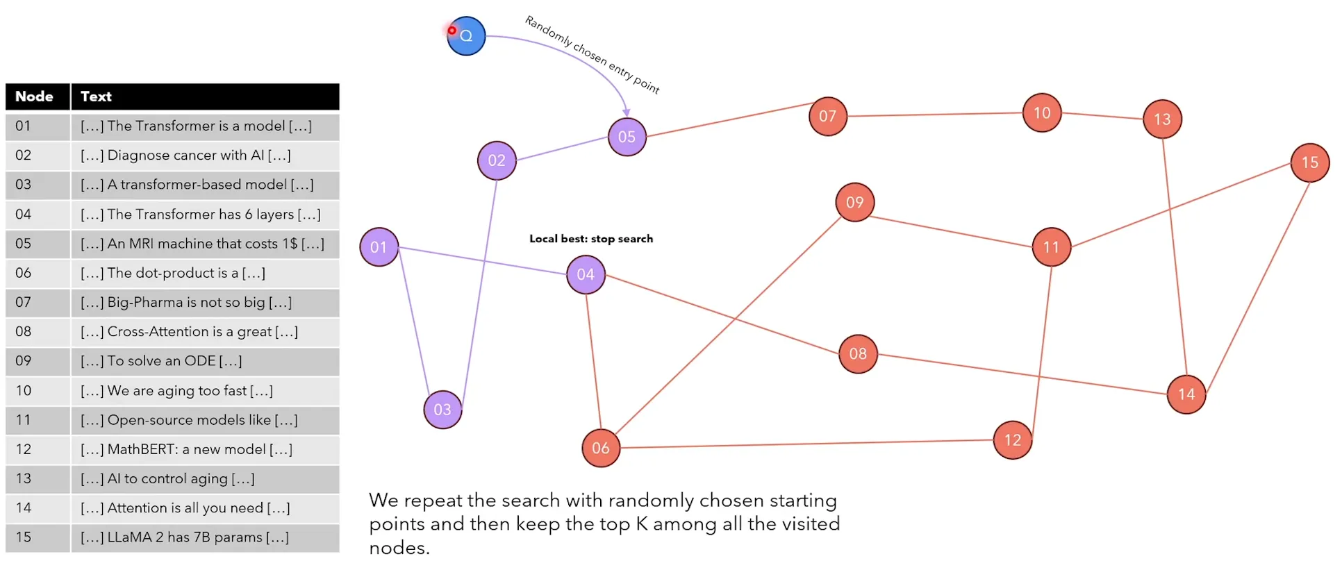
We’ll be looking into the Hierarchical Navigable Small Worlds(HNSQ) algorithm which is an extension of the Navigable Small Worlds proposal that states, every node is reachable from every node at a maximum of 6 steps. Let’s see it in example:

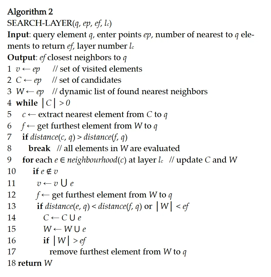
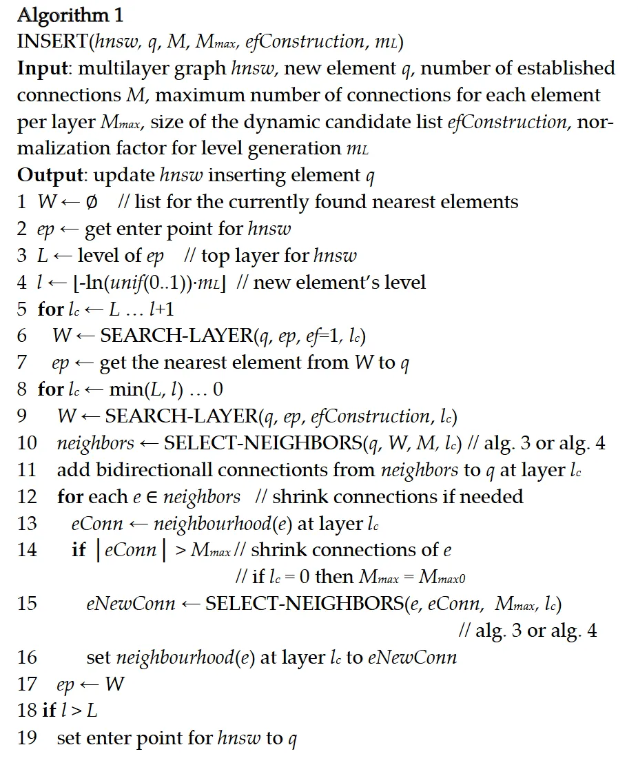
To find the node congaing the answer we want, we first start from a random node and then calculate the cosine similarity value between the query embedding and the value embedding stored in that node and its neighbors and we will continue to do this comparison until we reach to a node where the similarity score is not better. We repeat this steps to find the nodes with best values from each step and take the top k values of those best similarity scores.

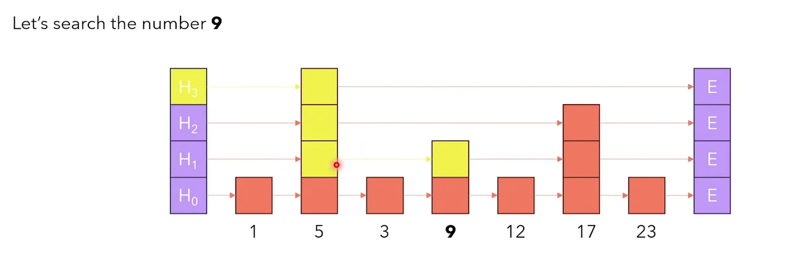
The Hierarchical part comes from the data structure we will use to implement the Hierarchical Navigable Small worlds algorithm, called Skip-List. Its a type of ds which the density of nodes decrease as we go up and we start our search from top to down left two right comparing values and bouncing back to left when ever we find larger values.

Lets see it in example: Here we started from the initial H3 which lands at 5 and since 9 > 5 we go right which bounce back to 5 after hitting end. Then we go one step down and go right and we hit 17 since 9 < 17 we know that our value is in the left so we bounce back to 5 and go down. The next value we hit is 9 and we found what we want. This is how skip-list works.

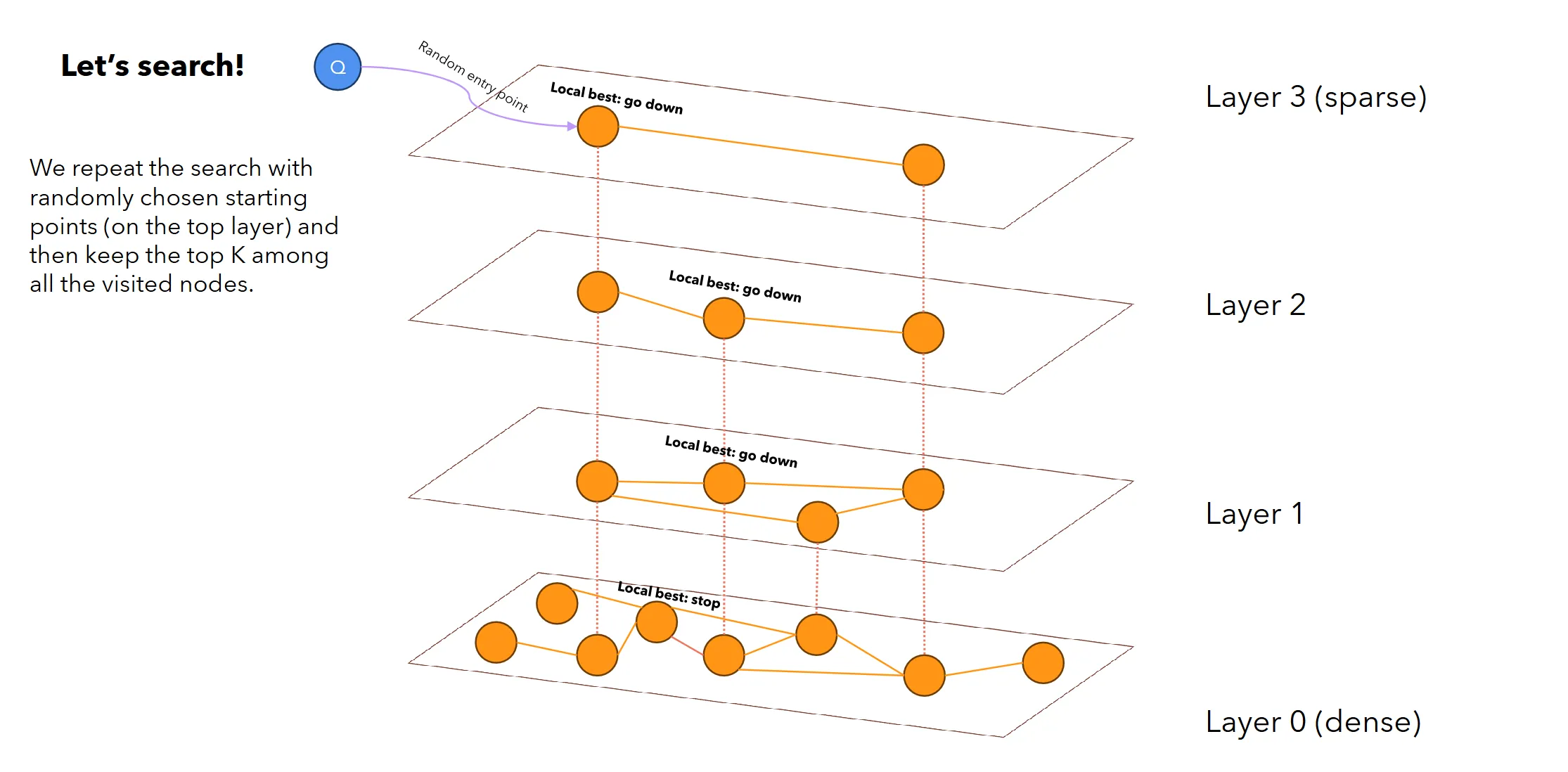
Now lets combine the idea of the skip list with the Navigable small worlds. The idea is to have layers containing nodes which go dense to sparce as we increase the layer and for each query we start from a random node from the top sparce node and we calculate and compare the similarity score with its neighbors and choose the one with higher and go down till we reach to the dense layer. We do this repeatedly and select the top k values of these nodes.

In order to add new nodes, we find nearest neighbor using our HNSW algorithm and add a node next to it based on its value.

References:

Reimers, Nils, and Iryna Gurevych. “Sentence-bert: Sentence embeddings using siamese bert-networks.” Proceedings of the 2019 conference on empirical methods in natural language processing and the 9th international joint conference on natural language processing (EMNLP-IJCNLP). 2019.

Malkov, Yu A., and Dmitry A. Yashunin. “Efficient and robust approximate nearest neighbor search using hierarchical navigable small world graphs.” IEEE transactions on pattern analysis and machine intelligence 42.4 (2018): 824-836.

Images: Umer Jamil slide on RAG.