Flash Attention

Heyy, lets now study how flash attention works from first principles. In this topic we will see:

The standard, self attention computation

1. Why we need Flash attention?

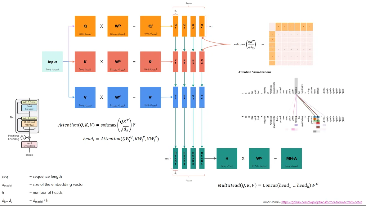
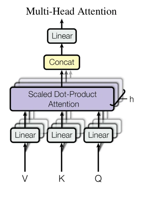
In transformer, we perform a multi head attention, which given a Query(Q), Key(K) and a value(V), each with a dimension of (seq len, num head)(N,d), then we multiply the Q * K^T, apply a softmax on it and then multiply with V. This will end us with multiple heads each containing part of the whole dimension, we then perform concatenation.

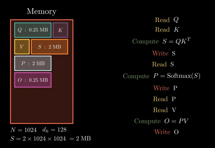
As the Q, K,V are huge matrix being stored at High Bandwidth Memory(HBM)(DRAM) of our gpu their attention computation involves frequent IO operation which makes the computation slower and expensive(O(N^2). There is another smaller and faster memory which is shared memory which we use to perform the actual multiplications. So the main question will be how can we reduce the frequency of IO operations by dividing our matrix into smaller ones in a way that fit the shared memory and perform the operations there.

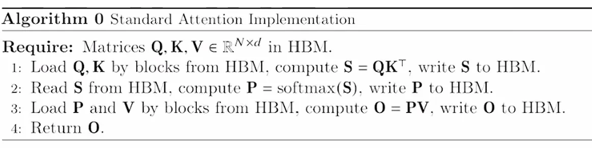
But in this blocked operation, computing the SoftMax of the Q*K^T will be a problem because it needs to access all the rows of this matrix multiplication to calculate the normalization factor which is the exponential of all items in row.

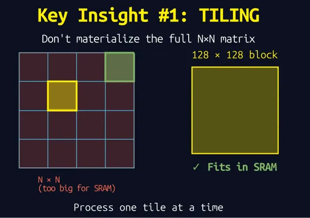
Instead of utilizing the full NXN matrix, we break our full matrix into smaller NxN version, which fits our SRAM and perform our operation efficiently.

2. Safe and Online softmax

Lets first see how we perform a SoftMax operation given a matrix R(N,N) which is a product of the Q * K^T:

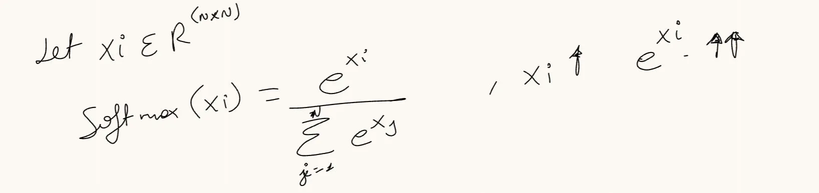
Since we’re computing the exponential, as the value of the xi becomes large the exponential of that number will become very large for example: if we say our xi was 100 its exponential is **26.9 tredecillion(**2.6881171418×10^43). Yep, tooo large and there is no way which we can represent this in our float16 or float32 precisely so it becomes numerically unstable.

In order to address this issue, we can introduce a variable into our computation, and make that variable the max value in the whole matrix which will reduce the operation between 0 and 1 since the xi value will be either negative or zero and the e^-x → e^0 lies between 0 and 1.

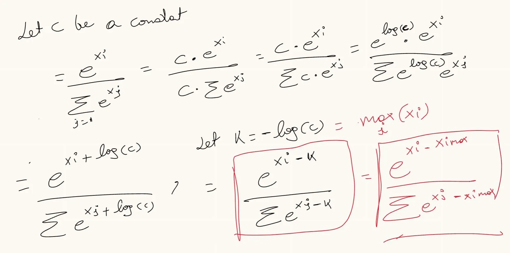
So our step will be:

1. Find the max value which takes O(N) time and memory
2. calculate the normalization factor : O(N) time and memory
3. divide each points by the normalization factor : another O(N) operation

So we will end up with three sequential operations which takes linear time and memory complexity, but we don’t like linear things in GPU right :) so we need to find a better way. That’s where the online softmax comes to the picture.

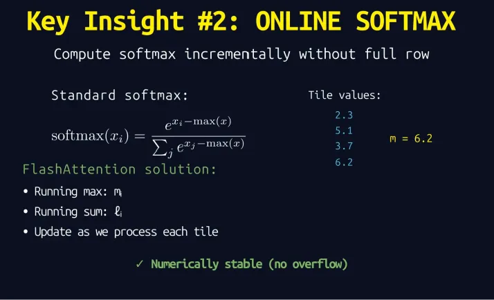
The goal here is combing the first two processes(finding the maximum and finding the normalization factor) into one step so we reduce the total step into two steps.

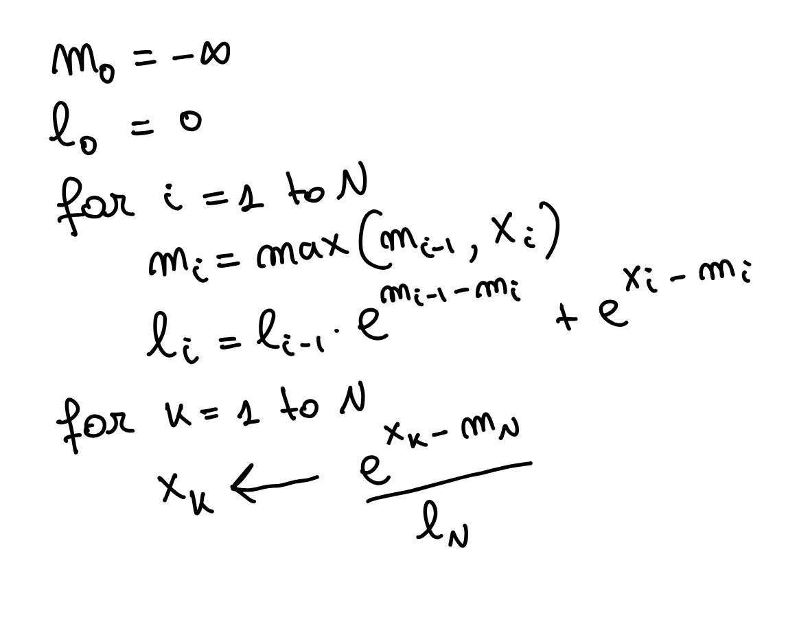
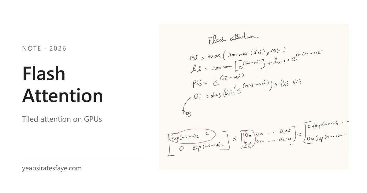
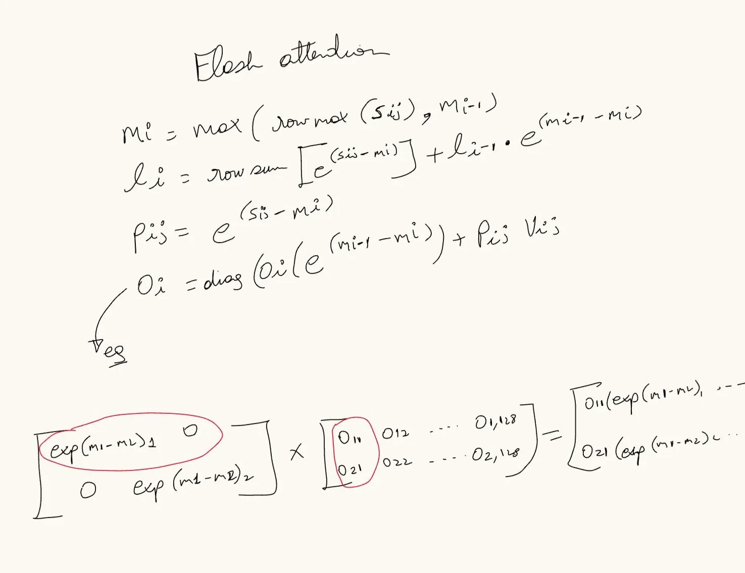
Find the local maximum and compute the normalization factor. When you’re computing the normalization factor of the previous step multiply it with a corrective factor which is made of the e^ of the previous maximum - the current maximum. If these two are same will result e^0 which is one without damage. This will help us finish the two operations on one pass.

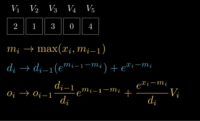
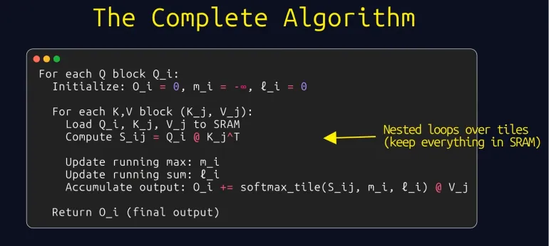
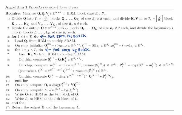
note that even though we’re no longer visiting the HBM twice, we’re still storing the SoftMax output into our HMB and read it as we need it for the weighted some computation. We can avoid this by adding the weighted sum into our running variables. This means for each row of multiplication will be updating, the running max, denominator and attention output. This will help us end up one weighted score for output at one pass of the memory read.

To do this, as we progress, we multiply our v by the ratio of the denotator (sum of the e^i-1 -i).

Specifically, after factoring out the denominator, its like multiplying the old output by the new denominator/ old denominator.

3. How block matrix multiplication works?

Its a way of dividing our matrices into blocks, and computing the results as a block. This help us parallelize the computation into multiple cores while keeping the results. When it comes to dividing our matrices, we can divide our matrix how every we want as long as the shape of the blocks is compatible to do the multiplication.

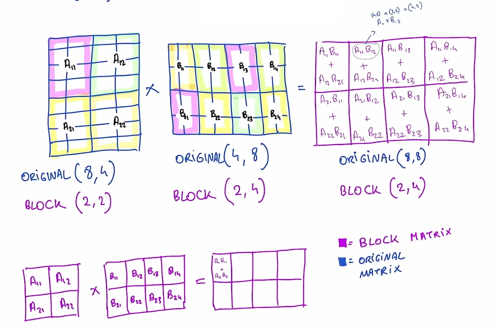
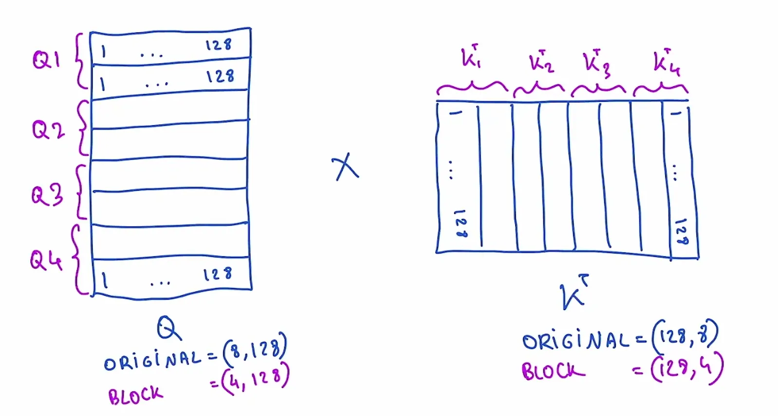
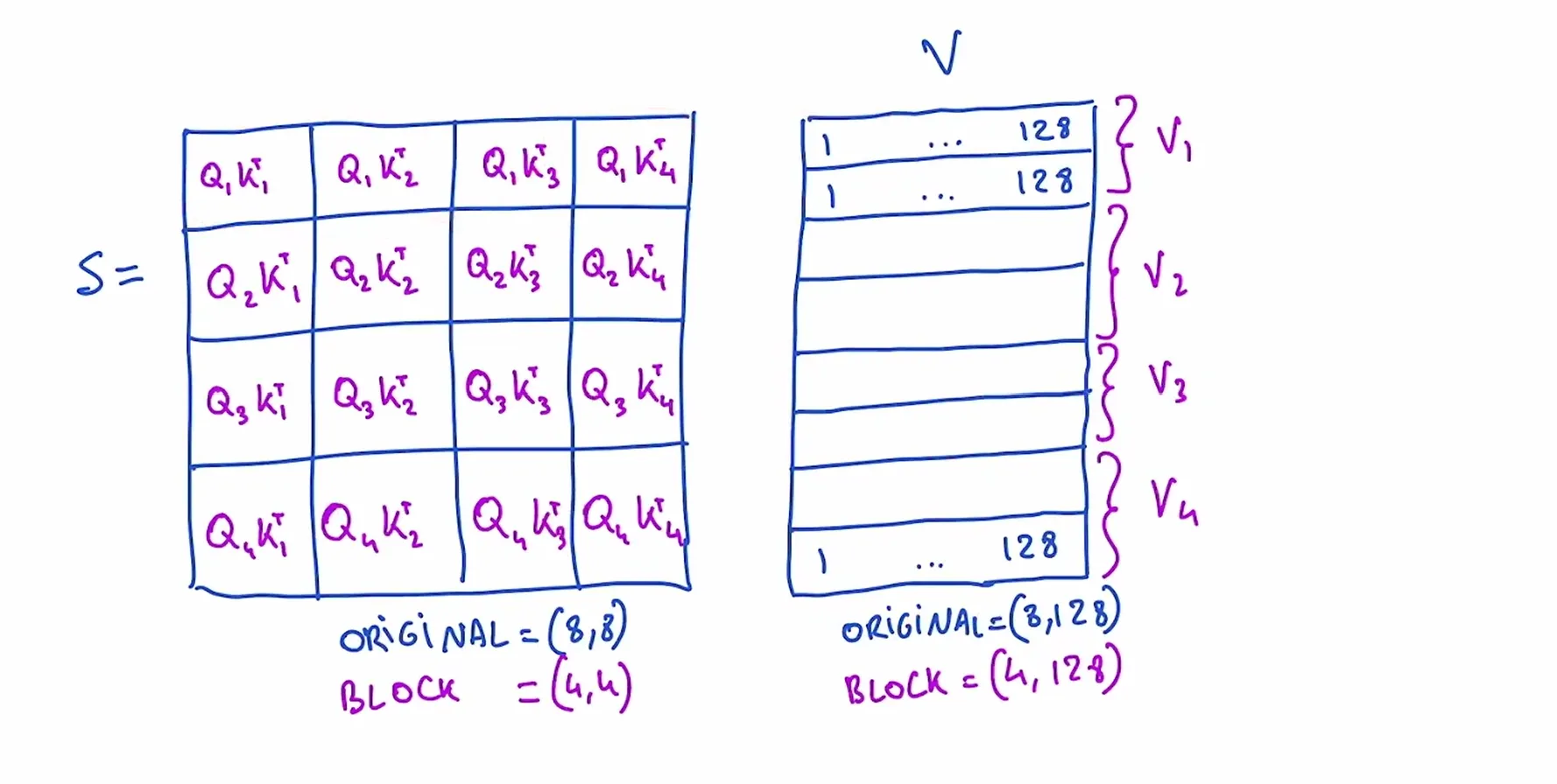
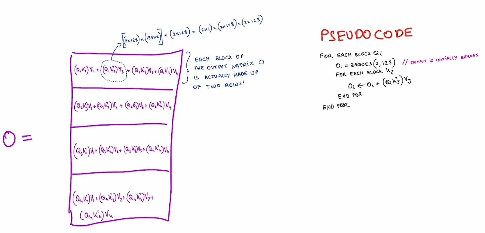
One thing we glanced over here while computing the Q * K^T is the SoftMax operation and in this block matrix multiplication operation, we’ll apply a SoftMax operation without the normalization step(exp. Which is:

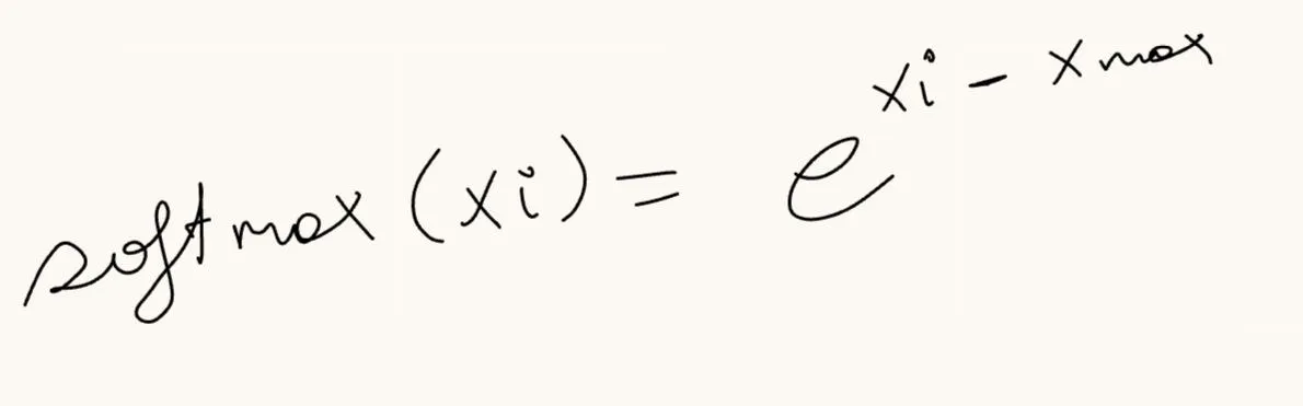
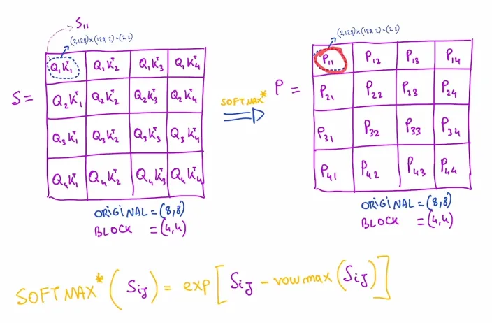
Note that the row max here is not the max for the entire row but the max for the local block, since each block is composed of a shape (2,128).

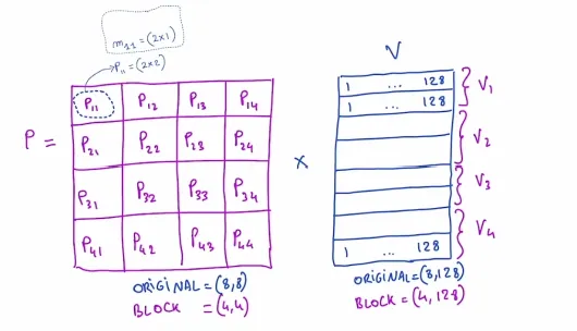
So we can fix this issue by applying our online SoftMax computation method, which we compute the local maximum to get the local softmax and apply a correction factor if we found another maximum. And also on the way calculate our global normalization factor in a same way we did.

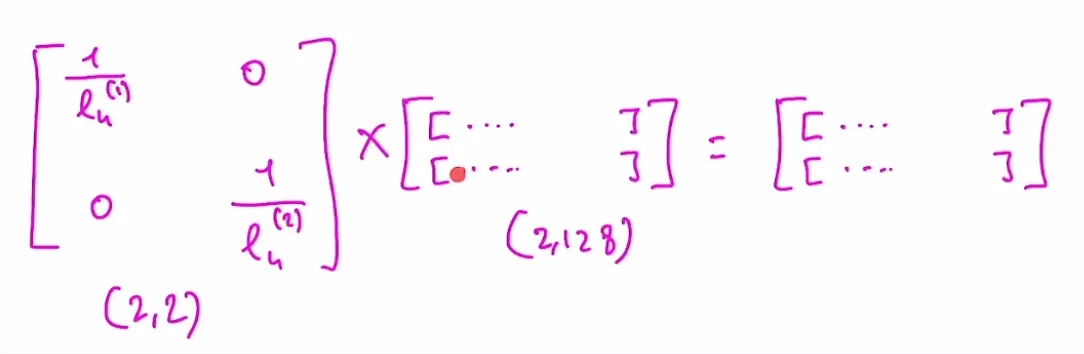
Once we’ve the last output value we can divide it by the normalization factor and have our softmax value.

4. Introduction to CUDA and GPU

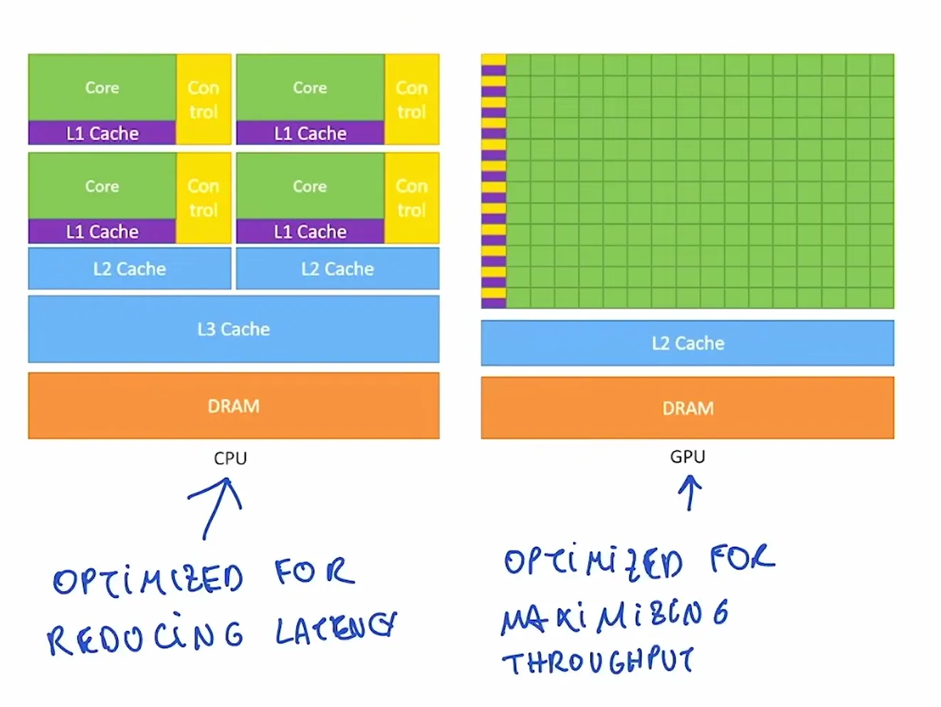
When we do operations on GPU we utilize multiple cores parallelly. The group of threads in our GPU is called Wrap and they share same control unit and cache and they work on same instruction at any time, but the value of our variables may differ.

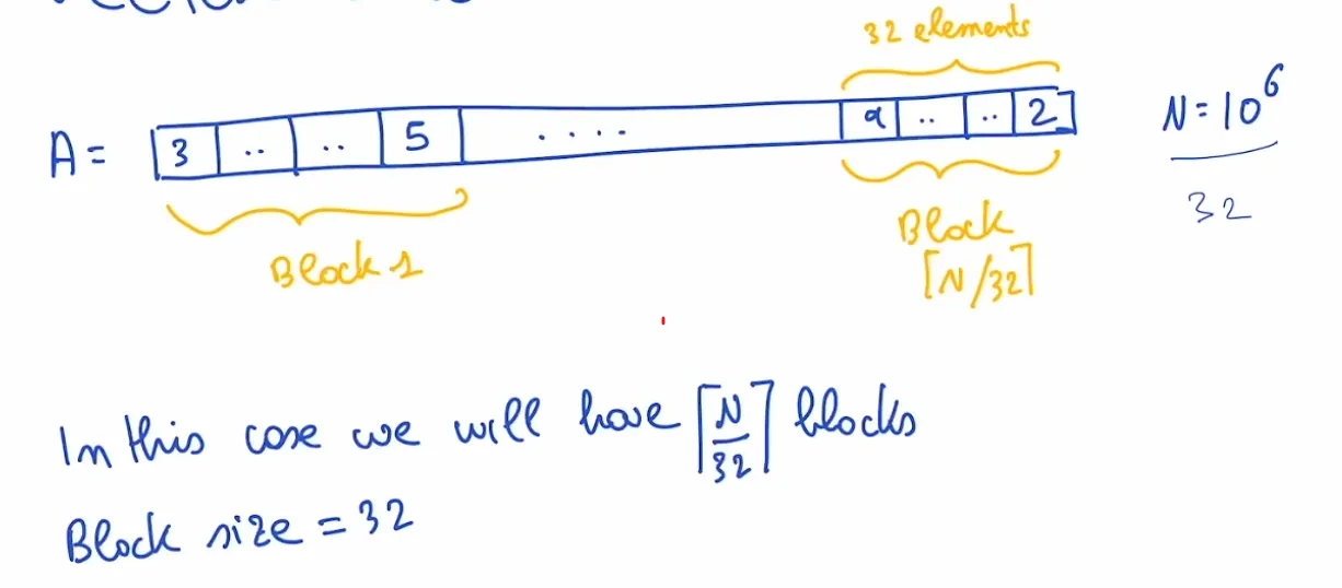
When we process a data that’s larger than our thread, we can divide our data into blocks. And our gpu will be processing blocks of data at a time. For example if we’ve a million data to process, we don’t have a million threads to process our data so we divide our data into blocks. Lets say our block size is 32, so we will have N/32 blocks to process. If our gpu has 64 cores it means it can process two blocks at a time.

We need to map which element should be processed by which thread by using

In our GPU, we’ve two types of memory the DRAM(global memory) which has larger size but slower access and shared memory belonging to all the threads in a same block, which is very small compared to the DRAM but has very fast access time. So the goal here will be how to utilize this faster shared memory and reduce our roundtrip to the global memory.

5. Autograd with a Jacobian

When we’re computing the gradient over our variables using the normal backpropagation, since we’ll be working with vectors with a very high dimension, our computation will be enormous.

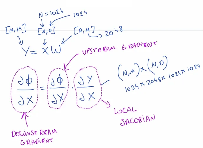
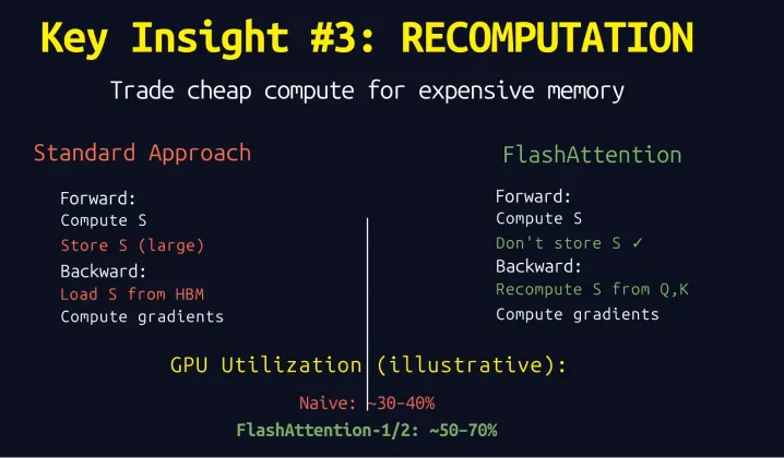
Instead of storing our computation during the froward pass and utilizing it into the backward pass, in the flash attention we will need to recompute the attentions same way as we did for the forward pass, this will cause higher utilization of computational resources while reducing our memory utilization. This will help us ultimate our memory bottleneck.

References

ExplainingAI - FlashAttention Explained from Scratch

Umar Jamil - Flash Attention derived and coded from first principles with Triton (Python)